Gradient descent is perhaps one of the most common optimization algorithms today. It performs updates of the form
\[x_{t + 1} = x_{t} - \eta_{t}\nabla L\left( x_{t} \right).\]
But it often suffers from slow convergence. To mitigate this, a common technique is to “change the metric” in which we perform gradient descent; to do so, first note that we can rewrite the usual gradient descent update as
\[\begin{aligned} x_{t + 1} & = x_{t} - \eta_{t}\nabla L\left( x_{t} \right) = \arg\min\limits_{x}\left( \underset{\text{ (i)}}{\underbrace{L\left( x_{t} \right) + {\langle\nabla L\left( x_{t} \right),x - x_{t}\rangle}}} + \frac{1}{2\eta_{t}}\underset{\text{ (ii)}}{\underbrace{\left\| {x - x_{t}} \right\|^{2}}} \right); \end{aligned}\] this can be easily checked by taking the gradient of the loss inside the argmin and equating it to zero. This gives us some great intuition on what gradient descent does: we are minimizing the first-order Taylor approximation of \(L\) around \(x_{t}\) (term (i)), while regularizing to ensure that we don’t stray too far from \(x_{t}\) (term (ii)); this is to keep the Taylor approximation sufficiently accurate. The learning rate determines the strength of this regularization.
But note that while \(\left\| {x - x_{t}} \right\|^{2}\) is a natural measure of distance, it is hardly the only one. Generally speaking, by replacing it with a different distance measure we obtain variants of gradient descent that may significantly improve convergence. For example, consider using the Mahalanobis metric with a symmetric positive matrix \(A\): \[x_{t + 1} = \arg\min\limits_{x}\left( L\left( x_{t} \right) + {\langle\nabla L\left( x_{t} \right),x - x_{t}\rangle} + \frac{1}{2\eta_{t}}\left( x - x_{t} \right)^{T}A\left( x - x_{t} \right) \right);\] the loss in the argmin is convex, so equating its gradient to zero we obtain that \[\begin{aligned} x_{t + 1} & = \arg\min\limits_{x}\left( L\left( x_{t} \right) + {\langle\nabla L\left( x_{t} \right),x - x_{t}\rangle} + \frac{1}{2\eta_{t}}\left( x - x_{t} \right)^{T}A\left( x - x_{t} \right) \right); \\ & \Longleftrightarrow \nabla L\left( x_{t} \right) + \frac{2}{2\eta_{t}}A\left( x_{t + 1} - x_{t} \right) = 0 \\ & \Longleftrightarrow A\left( x_{t + 1} - x_{t} \right) = - \eta_{t}\nabla L\left( x_{t} \right) \\ & \Longleftrightarrow x_{t + 1} = x_{t} - \eta_{t}A^{- 1}\nabla L\left( x_{t} \right). \end{aligned}\] This is often called “(linearly) preconditioned” gradient descent, with \(A^{- 1}\) referred to as the preconditioner.1 Naturally, \(A = I\) recovers usual gradient descent.
Using a preconditioner can substantially boost convergence. The classical example is with a quadratic loss function: consider the loss \[L(x) = \frac{1}{2}x^{T}\begin{pmatrix} 1.0 & 0.7 \\ 0.7 & 1.0 \end{pmatrix}x,\] which is convex and quadratic, and let us start optimization from \(x_{0} = ( - 1,3)\).
We’ll run three optimization algorithms:
Vanilla gradient descent;
Preconditioned gradient descent with preconditioner \(A^{- 1} = \begin{pmatrix} 2 & - 1 \\ - 1 & 2 \end{pmatrix}\); and
Preconditioned gradient descent with preconditioner \(B^{- 1} = \begin{pmatrix} 2 & 1 \\ 1 & 2 \end{pmatrix}\).
On all cases, we’ll tune the learning rates for best performance. The results are as follows:
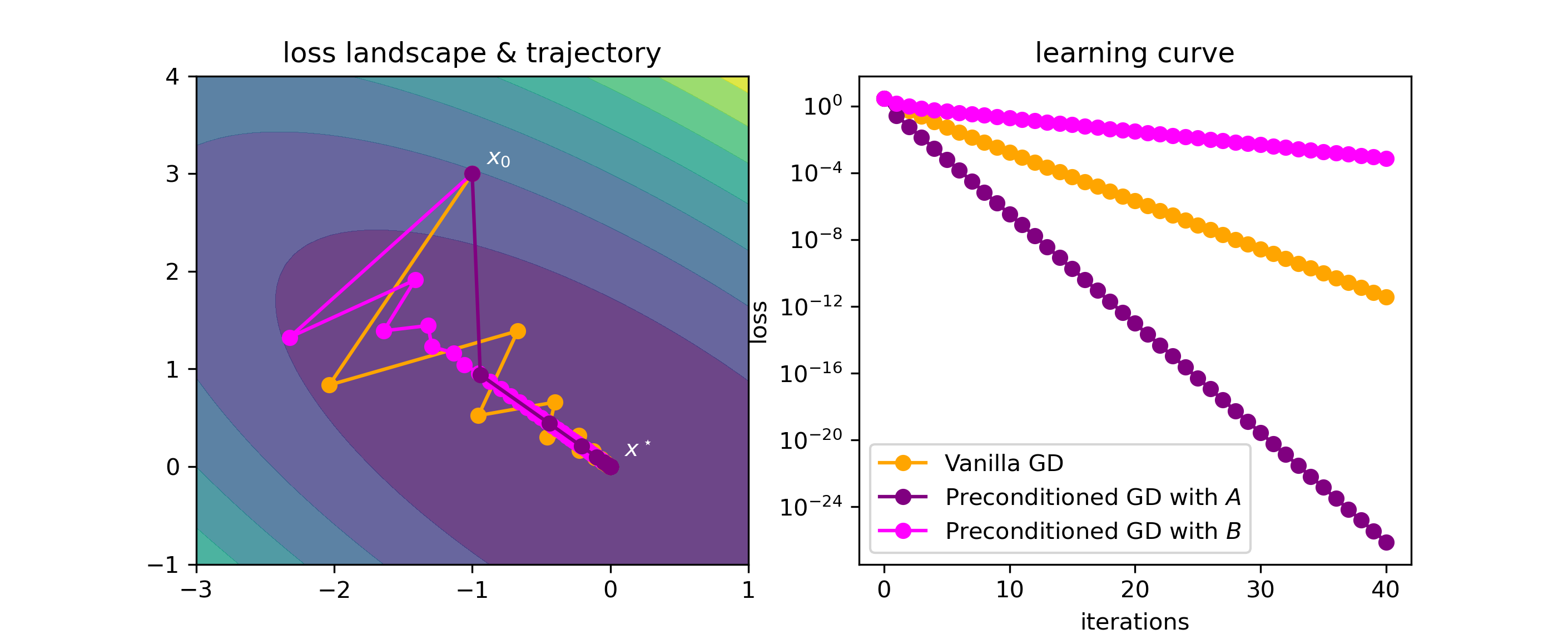
Figure: Optimization trajectory & learning curve for vanilla and preconditioned gradient descent.
As we can see, preconditioning can really help – the results with \(A^{- 1}\) as the preconditioner are orders of magnitude more accurate than without preconditioning! But we do need to be careful with our choice of preconditioner, as a bad preconditioner can be worse than no preconditioner at all (cf. \(B^{- 1}\) as the preconditioner).
So this raises the question: what is a good choice of preconditioner?
Detour: the inverse Hessian and Newton’s method
Common wisdom is that taking the preconditioner to equal or at least approximate the inverse Hessian at \(x_{t}\) is right about the best option. While this is not generally true (as we will see), I think it’s worth taking a brief detour to discuss a bit more on why one would think this.
In a gist, this choice of “preconditioned gradient descent” becomes Newton’s method for optimization. It performs updates of the form \[\begin{aligned} x_{t + 1} & = x_{t} - \eta_{t}\left( \nabla^{2}L\left( x_{t} \right) \right)^{- 1}\,\nabla L\left( x_{t} \right) \\ & = \arg\min\limits_{x}\left( L\left( x_{t} \right) + {\langle\nabla L\left( x_{t} \right),x - x_{t}\rangle} + \frac{1}{2\eta_{t}}\left( x - x_{t} \right)^{T}\left( \nabla^{2}L\left( x_{t} \right) \right)\left( x - x_{t} \right) \right), \end{aligned}\] which corresponds to minimizing the second-order Taylor approximation of \(L\) about \(x_{t}\), but without any regularization on the step size.
As one can perhaps imagine, this lack of regularization makes Newton’s method prone to convergence issues. Generally speaking, even with strongly convex loss functions it may diverge if the initial estimate \(x_{0}\) is too far from a local minimum. (There are variants such as cubic regularized Newton or damped Newton that resolve this, but this is beyond the scope of this post.)
But when Newton’s method converges, it does so quickly – in particular, much faster than vanilla gradient descent. Famously, while gradient descent obtains linear convergence rates, Newton’s method obtains quadratic convergence rates – a significant improvement.
That said, is Newton’s method “optimal” in some sense? Well, let’s consider what happens when we use it on a quadratic \[L(x) = \frac{1}{2}x^{T}Ax - x^{T}b;\] in this case, we have \[\nabla L(x) = Ax - b\quad\quad\text{ and }\quad\quad\nabla^{2}L(x) = A,\] and so the first Newton step with \(\eta_{0} = 1\) becomes \[x_{1} = x_{0} - A^{- 1}\left( Ax_{0} - b \right) = x_{0} - x_{0} + A^{- 1}b = A^{- 1}b = x^{\star}.\] So regardless of where we start, Newton’s method fully converges in a single step for quadratics. Well, this is clearly optimal – no method can converge faster than a single step. This factoid often leads some to believe that Newton’s method is more broadly optimal, but this is not so, as its lack of global convergence in more general settings already indicates. Note also that in the particular case of quadratics, the Hessian is constant wrt. \(x\), so in a sense the fact that Newton’s method works so well there is more about an “optimal (fixed) preconditioning” than actually doing Newton’s method (which involves continuously changing Hessians). So, with that in mind, let us explore preconditioners some more.
Nonlinear preconditioners
A first very useful step will be to slightly generalize what we are calling preconditioners, so as to support so-called “non-linear” preconditioners. Again viewing the update step as an argmin, the key will be to write it in the general form
\[x_{t + 1} = \arg\min\limits_{x}\left( L\left( x_{t} \right) + {\langle\nabla L\left( x_{t} \right),x - x_{t}\rangle} + \frac{1}{\eta_{t}}R\left( x - x_{t} \right) \right),\] where \(R:{\mathbb{R}}^{d} \rightarrow {\mathbb{R}}_{\geq 0}\) is any strictly convex differentiable function with minimum at \(R(0) = 0\) (the “regularizer”). \(R\) being strictly convex ensures that the loss in the argmin is itself strictly convex, and thus has a unique minimizer, and furthermore having its minimum at \(R(0) = 0\) ensures that \(R\left( x_{t} - x \right)\) is a coherent distance measure. Thanks to strict convexity we can solve for our update by equating the gradient of the loss in the argmin to zero:
\[\begin{aligned} x_{t + 1} & = \arg\min\limits_{x}\left( L\left( x_{t} \right) + {\langle\nabla L\left( x_{t} \right),x - x_{t}\rangle} + \frac{1}{\eta_{t}}R\left( x - x_{t} \right) \right) \\ & \Longleftrightarrow \nabla L\left( x_{t} \right) + \frac{1}{\eta_{t}}\nabla R\left( x_{t + 1} - x_{t} \right) = 0 \\ & \Longleftrightarrow \nabla R\left( x_{t + 1} - x_{t} \right) = - \eta_{t}\nabla L\left( x_{t} \right), \end{aligned}\] and because \(R\) is strictly convex its gradient \(\nabla R\) must admit a left-inverse \(\nabla R^{- 1}\), so \[\begin{aligned} & \nabla R\left( x_{t + 1} - x_{t} \right) = - \eta_{t}\nabla L\left( x_{t} \right) \\ & \Longleftrightarrow x_{t + 1} - x_{t} = \nabla R^{- 1}\left( - \eta_{t}\nabla L\left( x_{t} \right) \right) \\ & \Longleftrightarrow x_{t + 1} = x_{t} + \nabla R^{- 1}\left( - \eta_{t}\nabla L\left( x_{t} \right) \right). \end{aligned}\] This gives our update step in closed form, with \(\nabla R^{- 1}:{\mathbb{R}}^{d} \rightarrow {\mathbb{R}}^{d}\) being our (possibly nonlinear) preconditioner. Note how the learning rate and negation happen before the preconditioner, rather than afterwards as we typically write for linear preconditioners. But of course, both are equivalent in the linear case, since when the preconditioner is linear it commutes with scaling.
Optimal preconditioners
So our goal now is to, given a loss \(L\), know how to produce an ‘optimal” preconditioner \(R\).
The first matter we should settle is how to define optimality; there are many possible notions we could consider. For the purposes of this post we’ll consider the following, which we shall dub “one-step optimality”:
Definition (One-step optimality). A preconditioner \(\nabla R^{- 1}\) is one-step optimal for the loss \(L\) if, for any starting position \(x_{0}\), gradient descent on \(L\) preconditioned with \(\nabla R^{- 1}\) and with step \(\eta_{t} \equiv 1\) converges in a single step; i.e., \[x_{1} = x_{0} + \nabla R^{- 1}\left( - \nabla L\left( x_{0} \right) \right) = x^{\star},\quad\text{ for every }x_{0} \in {\mathbb{R}}^{d}.\]
This is a very strong condition! But note that if we are able to satisfy it, then we automatically satisfy most other reasonable notions of optimality for fixed \(L\) (e.g., minimum number of steps until \(\varepsilon\)-close to convergence). Note that the step sizes \(\eta_{t}\) is taken to equal one as otherwise the one-step optimal preconditioner may (and generally would) need to “annul“/compensate it.
With this definition in hand, it is actually pretty simple to derive the form of one-step optimal preconditioners. Indeed, it follows that \(\nabla R^{- 1}\) is one-step optimal iff, for all \(x \in {\mathbb{R}}^{d}\),
\[\nabla R^{- 1}\left( - \nabla L(x) \right) = x^{\star} - x.\]
I.e., the optimal preconditioner “undoes” the negative gradient (thus obtaining \(x\)) and then points in the direction of \(x^{\star}\) (which is fixed). Let’s formalize this: suppose that the loss \(L\) is strictly convex. This ensures that the gradient \(\nabla L\) admits a (bijective) left-inverse \(\nabla L^{- 1}\), with which we can define
\[\nabla R_{\text{opt-}L}^{- 1}(d) ≔ x^{\star} - \nabla L^{- 1}( - d).\]
It is straightforward to show that \(\nabla R_{\text{opt-}L}^{- 1}\) is (i) one-step optimal, and (ii) under mild conditions, the unique one-step optimal preconditioner.
Proposition. Let \(L\) be strictly convex. Then \(\nabla R_{\text{opt-}L}^{- 1}\) is one-step optimal. If \(L\) is coercive, then \(\nabla R_{\text{opt-}L}^{- 1}\) is furthermore unique.
Proof: It’s trivial to show that \(\nabla R_{\text{opt-}L}^{- 1}\) is one-step optimal: \[\nabla R_{\text{opt-}L}^{- 1}\left( - \nabla L(x) \right) = x^{\star} - \nabla L^{- 1}\left( \nabla L(x) \right) = x^{\star} - x.\] Now, to show uniqueness, suppose \(\nabla R_{\text{other}}^{- 1}\) is some other one-step optimal preconditioner, different from \(\nabla R_{\text{opt-}L}^{- 1}\). Then \[\nabla R_{\text{opt-}L}^{- 1}\left( - \nabla L(x) \right) = x^{\star} - x = \nabla R_{\text{other}}^{- 1}\left( - \nabla L(x) \right).\] But this means that \(\nabla R_{\text{opt-}L}^{- 1}\) and \(\nabla R_{\text{other}}^{- 1}\) must agree on the range of \(- \nabla L\), and so it must be unique when constrained to this range. When \(L\) is coercive, its range equals the whole domain, rendering \(R_{\text{opt} - L}^{- 1}\) unique.
□For completeness sake, let us also write down who \(\nabla R\) and \(R\) must be.
\[\begin{aligned} \nabla R^{- 1}(d) = x^{\star} - \nabla L^{- 1}( - d) & \Longleftrightarrow d = \nabla R\left( x^{\star} - \nabla L^{- 1}( - d) \right) \\ & \Longleftrightarrow - \nabla L(d) = \nabla R\left( x^{\star} - \nabla L^{- 1}\left( \nabla L(d) \right) \right) \\ & \Longleftrightarrow - \nabla L(d) = \nabla R\left( x^{\star} - d \right) \\ & \Longleftrightarrow \nabla L(d) - x^{\star} = \nabla R(d), \end{aligned}\] and \[\begin{aligned} \nabla R(d) = \nabla L(d) - x^{\star} & \Longleftrightarrow R(d) = L(d) - \langle x^{\star},d\rangle; \end{aligned}\] note that \(R\) is indeed strictly convex, since we assumed \(L\) is strictly convex.
It is also not too hard to prove – though perhaps a bit unfortunate – that the existence of one-step optimal preconditioners2 is actually predicated on strict convexity of \(L\).
Proposition. Given a loss \(L\), there exists a one-step optimal preconditioner \(\nabla R^{- 1}\) for \(L\) if and only if \(L\) is strictly convex.
Proof: \(( \Longleftarrow )\) already shown in the previous proposition.
\(( \Longrightarrow )\) If it exists, we know that the one-step optimal preconditioner must have the form \[R(d) = L(d) - \langle x^{\star},d\rangle,\] and by definition must be strictly convex. But \(R\) is strictly convex if and only if \(L\) is.
□Though it is perhaps already remarkable that such a strong optimality condition can be satisfied for any strictly convex optimization problem.
So, now we know how to identify the unique one-step optimal preconditioner \(\nabla R^{- 1}\), as well as whether it exists. Now let’s see some concrete examples.
Example 1: quadratics
Let’s start by considering a quadratic \(L(x) = \frac{1}{2}x^{T}Ax - b^{T}x\), with \(A\) positive definite. Then:
\[\nabla L(x) = Ax - b,\quad\text{ and }\quad\nabla L^{- 1}(y) = A^{- 1}(y + b),\]
and so the one-step optimal preconditioner is given by \[\nabla R_{\text{opt-}L}^{- 1}(d) = x^{\star} - \nabla L^{- 1}( - d) = A^{- 1}b - A^{- 1}( - d + b) = A^{- 1}d,\] and we recover Newton’s method.
Example 2: mean estimation
Now let’s consider a simple statistical task: inferring a mean \({\mathbb{E}}\lbrack Y\rbrack\). This can be written as the minimization of the mean squared error \[L(x) = {\mathbb{E}}\left\lbrack \frac{1}{2}(x - Y)^{2} \right\rbrack.\] Then:
\[\nabla L(x) = x - {\mathbb{E}}\lbrack Y\rbrack,\quad\text{ and }\quad\nabla L^{- 1}(y) = y + {\mathbb{E}}\lbrack Y\rbrack.\]
Therefore, the one-step optimal preconditioner is given by
\[\nabla R_{\text{opt} - L}^{- 1}(d) = x^{\star} - \nabla L^{- 1}( - d) = {\mathbb{E}}\lbrack Y\rbrack - \left( - d + {\mathbb{E}}\lbrack Y\rbrack \right) = d,\]
so using no preconditioner is optimal here. (Of course, this is just another case of a quadratic.)
Example 3: maximum likelihood for Bernoulli data
Finally, let us consider a slightly more interesting example: maximum likelihood (i.e., minimizing cross-entropy) over a Bernoulli model, with the probability parameter parametrized through a sigmoid.
\[\begin{aligned} L(\theta) & = {\mathbb{E}}\left\lbrack - Y\log\sigma(\theta) - (1 - Y)\log\left( 1 - \sigma(\theta) \right) \right\rbrack \\ & = {\mathbb{E}}\left\lbrack - Y\log\sigma(\theta) - (1 - Y)\log\sigma( - \theta) \right\rbrack, \end{aligned}\] for \[\sigma(t) = \frac{1}{1 + e^{- t}}.\]
We then have
\[\begin{aligned} \nabla L(\theta) & = {\mathbb{E}}\left\lbrack - Y\nabla\log\sigma(\theta) - (1 - Y)\nabla\log\sigma( - \theta) \right\rbrack \\ & = {\mathbb{E}}\left\lbrack - Y\frac{\sigma(\theta)\sigma( - \theta)}{\sigma(\theta)} + (1 - Y)\frac{\sigma( - \theta)\sigma(\theta)}{\sigma( - \theta)} \right\rbrack \\ & = {\mathbb{E}}\left\lbrack - Y\sigma( - \theta) + (1 - Y)\sigma(\theta) \right\rbrack \\ & = {\mathbb{E}}\left\lbrack (1 - Y)\sigma(\theta) - Y\sigma( - \theta) \right\rbrack; \end{aligned}\] and, using the fact that \(Y \sim \text{ Bern}\left( p^{\star} \right)\) for some \(p^{\star} \in \lbrack 0,1\rbrack\), \[\begin{aligned} \nabla L(\theta) & = {\mathbb{E}}\left\lbrack (1 - Y)\sigma(\theta) - Y\sigma( - \theta) \right\rbrack; \\ & = \left( 1 - p^{\star} \right)\sigma(\theta) - p^{\star}\sigma( - \theta) \\ & = \left( 1 - p^{\star} \right)\sigma(\theta) - p^{\star}\left( 1 - \sigma(\theta) \right) \\ & = \left( 1 - p^{\star} \right)\sigma(\theta) - p^{\star} + p^{\star}\sigma(\theta) \\ & = \sigma(\theta) - p^{\star}; \end{aligned}\] thus \[\nabla L^{- 1}(y) = \text{ logit}\left( y + p^{\star} \right),\] where \[\text{ logit}(t) = \sigma^{- 1}(t) = \log\frac{t}{1 - t}.\]
The one-step optimal preconditioner is therefore given by \[\nabla R_{\text{opt} - L}^{- 1}(d) = x^{\star} - \nabla L^{- 1}( - d) = \text{ logit}\left( p^{\star} \right) - \text{ logit}\left( - d + p^{\star} \right).\]
Closing thoughts: hardness and robustness of one-step optimal preconditioners
Of course, throughout all these examples one thing is clear: computing the one-step optimal preconditioner is generally as hard as solving the optimization problem itself. This is for a couple of reasons:
For one, the solution \(x^{\star}\) literally appears in the general form of the optimal preconditioner.
Even if \(x^{\star}\) wasn’t there, \(\nabla L^{- 1}( \cdot )\) also plays a fundamental role. But if we knew how to compute \(\nabla L^{- 1}( \cdot )\), then we would just compute \(\nabla L^{- 1}(0)\) and get \(x^{\star}\)!
These are indeed severe limitations. But, fortunately, the preconditioner’s role is just to speed up convergence; if it is incorrectly specified, we will still converge, only perhaps a bit slower. So here’s one pragmatic way to leverage our results so far: guess or estimate \(\nabla L^{- 1}( \cdot )\) (let’s call this estimate \(\nabla{\hat{L}}^{- 1}( \cdot )\), with the hat), and use \[\nabla{\hat{R}}^{- 1}(d) = \nabla{\hat{L}}^{- 1}(0) - \nabla{\hat{L}}^{- 1}(d).\] In certain cases (such as the Bernoulli MLE example) it suffices to have an estimate of the optimum, \(\theta^{\star}\).
It’s not too hard to see that a slightly misspecified optimal preconditioner generally isn’t too bad, especially if the learning rate \(\eta_{t}\) is slightly decreased. Indeed, at the \(t\)-th step:
\[\begin{aligned} & \left\| {\left( x_{t} - \nabla R^{- 1}\left( - \eta_{t}\nabla L\left( x_{t} \right) \right) \right) - \left( x_{t} - \nabla{\hat{R}}^{- 1}\left( - \eta_{t}\nabla L\left( x_{t} \right) \right) \right)} \right\| \\ & = \left\| {\nabla R^{- 1}\left( - \eta_{t}\nabla L\left( x_{t} \right) \right) - \nabla{\hat{R}}^{- 1}\left( - \eta_{t}\nabla L\left( x_{t} \right) \right)} \right\| \\ & = \left\| \begin{aligned} & \left( \nabla R^{- 1}(0) - \int_{0}^{1}\eta_{t}\nabla^{2}R^{- 1}\left( - s\eta_{t}\nabla L\left( x_{t} \right) \right)\nabla L\left( x_{t} \right)ds \right) \\ & \quad - \left( \nabla{\hat{R}}^{- 1}(0) + \int_{0}^{1}\eta_{t}\nabla^{2}{\hat{R}}^{- 1}\left( - s\eta_{t}\nabla L\left( x_{t} \right) \right)\nabla L\left( x_{t} \right)ds \right) \end{aligned} \right\| \\ & = \eta_{t}\left\| {\int_{0}^{1}\nabla^{2}R^{- 1}\left( - s\eta_{t}\nabla L\left( x_{t} \right) \right)\nabla L\left( x_{t} \right)ds - \int_{0}^{1}\nabla^{2}{\hat{R}}^{- 1}\left( - s\eta_{t}\nabla L\left( x_{t} \right) \right)\nabla L\left( x_{t} \right)ds} \right\| \\ & = \eta_{t}\left\| {\int_{0}^{1}\left( \nabla^{2}R^{- 1}\left( - s\eta_{t}\nabla L\left( x_{t} \right) \right) - \nabla^{2}{\hat{R}}^{- 1}\left( - s\eta_{t}\nabla L\left( x_{t} \right) \right) \right)\nabla L\left( x_{t} \right)ds} \right\| \\ & \leq \eta_{t}\int_{0}^{1}\left\| {\left( \nabla^{2}R^{- 1}\left( - s\eta_{t}\nabla L\left( x_{t} \right) \right) - \nabla^{2}{\hat{R}}^{- 1}\left( - s\eta_{t}\nabla L\left( x_{t} \right) \right) \right)\nabla L\left( x_{t} \right)} \right\| ds \\ & \leq \eta_{t}\left\| {\nabla L\left( x_{t} \right)} \right\|\int_{0}^{1}\left\| {\nabla^{2}R^{- 1}\left( - s\eta_{t}\nabla L\left( x_{t} \right) \right) - \nabla^{2}{\hat{R}}^{- 1}\left( - s\eta_{t}\nabla L\left( x_{t} \right) \right)} \right\|_{\text{op }}ds; \end{aligned}\] so as long as the operator norm within the integral is uniformly upper bounded, using the estimated optimal preconditioner should work pretty well.
Indeed, we can see this in practice. Here are some results on the Bernoulli MLE task, varying the choice of \(\theta^{\star}\) in the form of the optimal preconditioner, for data coming from \(\text{Bern}(0.3)\):
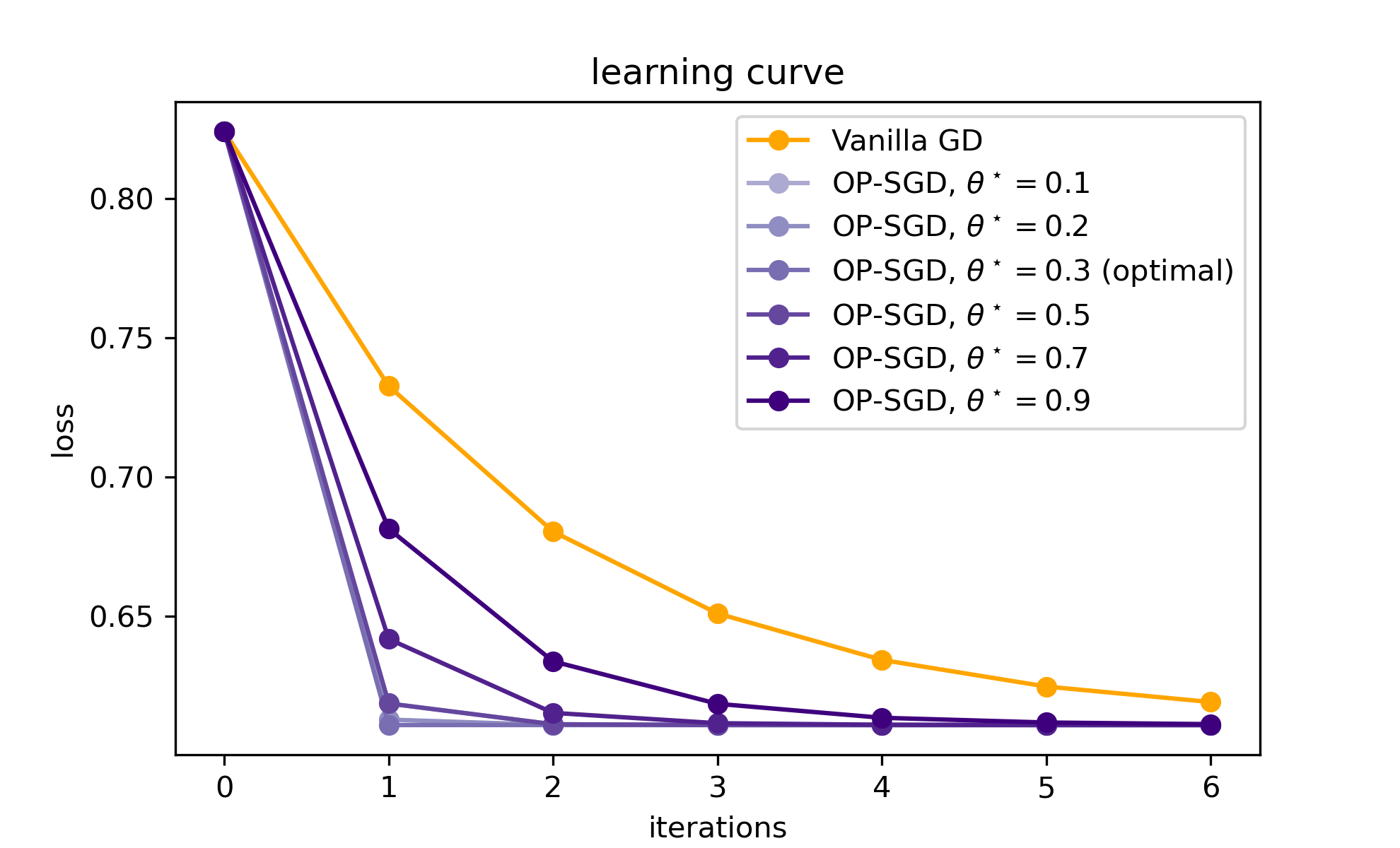
Figure: Learning curves for vanilla and (quasi-)optimally preconditioned gradient descent (OP-SGD), for various choices of \(p^{\star}\) of the preconditioner. Note how the preconditioned variants consistently beat vanilla gradient descent, even when the preconditioner is horribly misspecified.
This is a taste of the potential of preconditioners for gradient descent, and specifically of optimal/approximately-optimal ones. In a future post I intend to present a little bit more of the theory of optimal preconditioners, particularly regarding convergence. Another topic of particular interest, also for a future blog post, is the case of linear preconditioners; as it turns out, you can go quite far with them, as long as you weaken the notion of optimality a little bit. Stay tuned.
This can also be more broadly seen as an instance of mirror descent.↩︎
Within our nonlinear preconditioner framework, and for our particular definition of one-step optimal preconditioners.↩︎
If for some reason you'd like to cite this post, you can use this BibTeX entry (click to copy to clipboard).